
One of the most exciting things about artificial intelligence is the capability to predict. Though these models still contain some degree of error, scientists are constantly working on better models and on collecting more data to diminish the prediction error as much as possible. Today we use these models to predict the stock market, the weather, the price of real estate, machine failure and so much more within certain degrees of error. This information helps us to make better decisions.
Why?
Because the model captures multiple data points that might affect the variable we want to predict. Models are created by isolating variables or features that we feel contribute to the behavior of interest and figuring out some mathematical relationship between them.
Regression does exactly this. Regression is a statistical method that is used to predict a variable of interest (the variable we want to predict) Y by determining the strength and the kind of relationship this variable has with other independent variables, that are also referred to as features.
There are multiple types of regression and they are all used in different scenarios where the relationship between the dependent and independent variables tends to take on a specific form.
Types of Regression
Below you can see some basic types of regression.
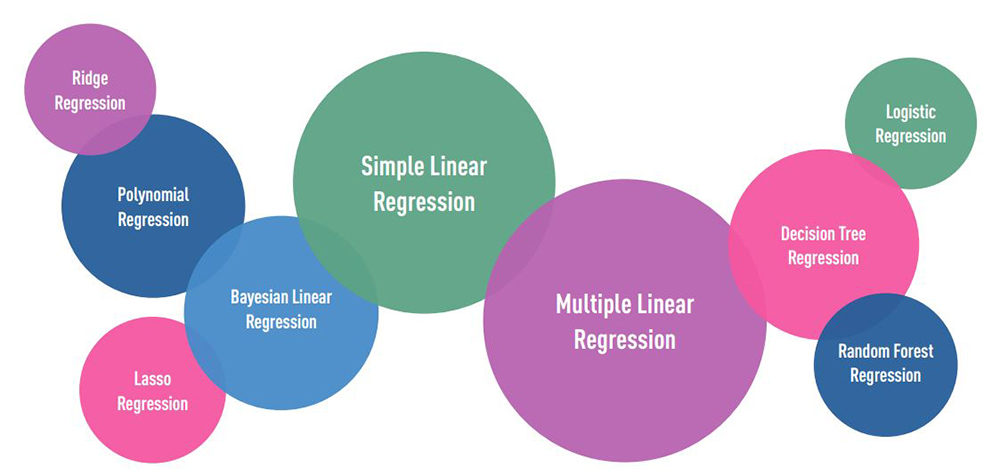
Basic Fitting
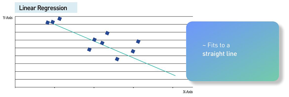

For instance in linear regression we are looking at a variable we want to predict, Y, that depends on only one more variable X. Their relationship is linear, that is it can be shown using a straight line.
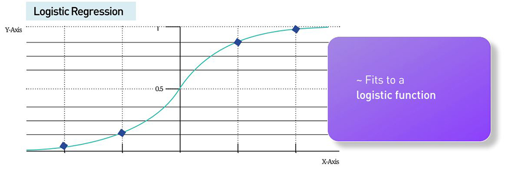
In polynomial regression the equation that relates X and Y is not linear but instead includes higher powers of X and hence ends up as a polynomial equation. The same logic holds true for logistic regression, where X and Y are related through a logistic function.
It is also possible to increase the number of variables that determine our independent variable Y. And so by changing the number of features (X1,X2,X3…) that determine Y, we need more complicated regression models.
In this article we want to work through a couple of examples so that you can really decode what’s going on. We will look at a couple of simple regression types.
The two most basic types of regression are simple linear regression and multiple linear regression. There are many more complicated regression methods but for this tech explainer we will focus on the two mentioned above.
In simple linear regression the premise is that we are looking for the relationship between one variable of interest and one other variable that we feel influences it. This is a very simple example and not one that practically fits life around us – this is used in very controlled experiments. But it is a great way to understand what is going on.
The general form of each type of regression under discussion:
1. Simple linear regression: Y = a + bX + u
2. Multiple linear regression:
Y = a + b1 X1 + b2 X2 + b3 X3 + … + bt Xt + u
For instance consider a variable of interest – real estate prices. We could say that the price of the house depends on the covered area of the house. The bigger the house the more expensive it is.
Our Model: Y = a + bX + u
This is actually the equation for a straight line, y = mx + c with the added residual error u. We have to incorporate this value to make sure we remember that our model will predict within a certain range. By keeping the residual error low we limit this range but it still exists and we must not forget that.
1. Y = the variable that we are trying to predict, in this case house price.
2. X = the variable we are using to predict Y, in this case the covered area.
3. a = the intercept.
4. b = the slope.
5. u = the regression residual.
Here Y is the price of the house, X is the covered area, u is an error term and a and b are the constants we need to find. ‘a’ is the Y intercept, the point where our line crosses the Y axis and ‘b’ is the gradient or the slope of the line.
Once we find these we can then find out the price for a house just given the covered area.
Let’s see this in action on an actual problem.
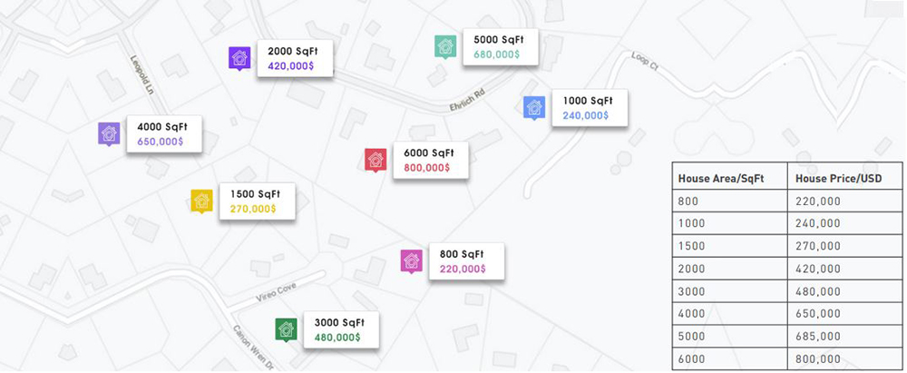
We start with a dataset where we have both the X and Y values. This is called the ‘training data’. Consider this data set. We have gathered some real estate data where we have the price of the house and area.
(Please note this is dummy data).
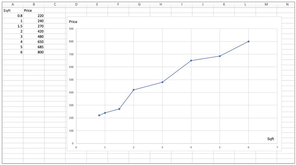
The next step is to find the line that passes as close to all our data points as possible. As you can see in the example below there are lots of lines possible.
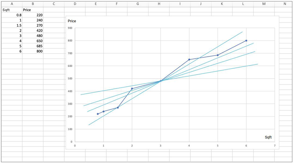
We have to find the one closest to ALL the data points. This is done by minimizing the difference between the actual data coordinate and the line for our model. We do this by minimizing the total distance of all the points from our model line. To make sure we penalize larger distances we take the squares of the distances instead of the actual distance. So the further the real point is from our model line, the more it will be penalized.
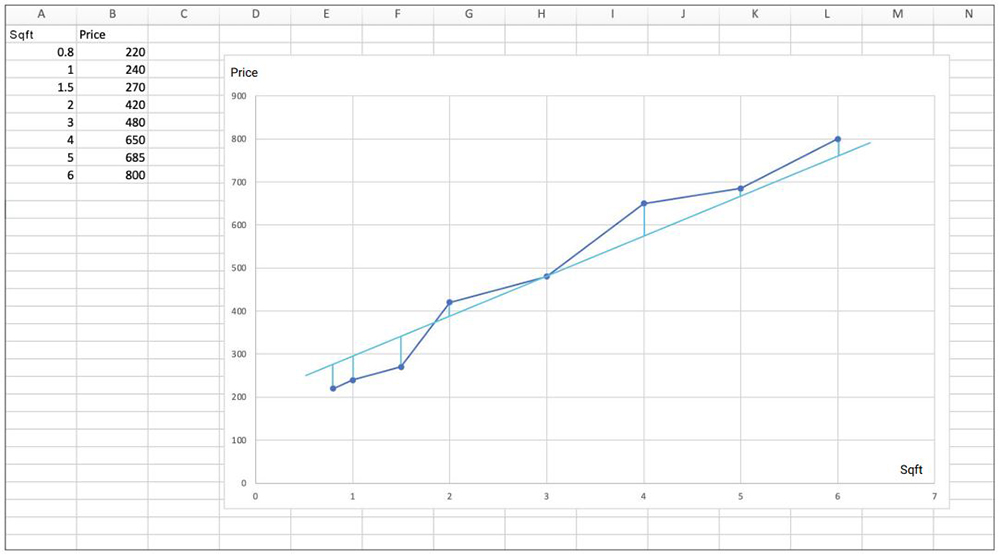
The error is defined as the difference between the real data point and the value given us by our model:
y-yi
Where y = axi + b
So axi + b -yi is the error and the error squared is (axi +b – yi)^2 The sum of these errors across n data points is:


This is great in theory but we all know that covered area is not the only thing that influences the price of a house. In reality there could be several other factors.
1. Number of bedrooms
2. Neighborhood
3. Covered area
4. Location within the community (close to a club, park etc)
What do we do then?
END OF PART 1


